Create and edit pivot tables
Pivot tables allow you to group and arrange data of large data sets to get summarized information. You can reorganize data in many different ways to display only the necessary information and focus on important aspects.
Create a new pivot table
To create a pivot table,
-
Prepare the source data set you want to use for creating a pivot table. It should include column headers. The data set should not contain empty rows or columns.
-
Select any cell within the source data range.
-
Switch to the Pivot Table tab of the top toolbar and click the Insert Table
 icon.
icon.
If you want to create a pivot table on the base of a formatted table, you can also use the  Insert pivot tableoption on the Table settings tab of the right sidebar.
-
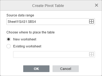
The Create Pivot Table window will appear.
-
The Source data range is already specified. In this case, all data from the source data range will be used. If you want to change the data range (e.g. to include only a part of source data), click the icon. In the Select Data Range window, enter the necessary data range in the following format: Sheet1!$A$1:$E$10. You can also select the necessary cell range on the sheet using the mouse. When ready, click OK.
-
Specify where you want to place the pivot table.
-
The New worksheet option is selected by default. It allows you to place the pivot table in a new worksheet.
-
You can also select the Existing worksheet option and choose a certain cell. In this case, the selected cell will be the upper right cell of the created pivot table. To select a cell, click the
 icon.
icon.
In the Select Data Range window, enter the cell address in the following format: Sheet1!$G$2. You can also click the necessary cell in the sheet. When ready, click OK.
-
-
-
When you select the pivot table location, click OK in the Create Tablewindow.
The Pivot table settings tab on the right sidebar will be opened. You can hide or display this tab by clicking the  icon.
icon.
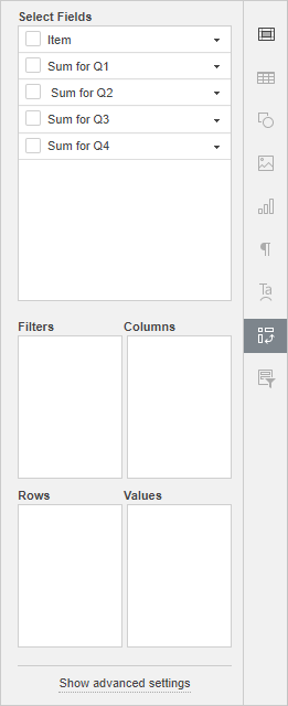
Select fields to display
-
If you add a field to the Filters section, a separate filter will be added above the pivot table. It will be applied to the entire pivot table. If you click the dropdown arrow
 in the added filter, you'll see the values from the selected field. When you uncheck some values in the filter option window and click OK, the unchecked values will not be displayed in the pivot table.
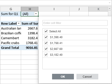
-
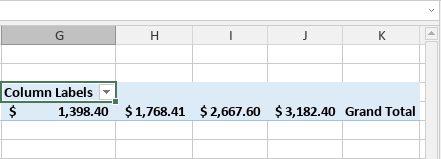
If you add a field to the Columns section, the pivot table will contain a number of columns equal to the number of values from the selected field. The Grand Total column will also be added.
-
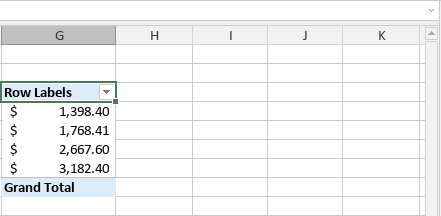
If you add a field to the Rows section, the pivot table will contain a number of rows equal to the number of values from the selected field. The Grand Total row will also be added.
-
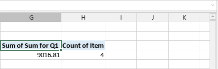
If you add a field to the Values section, the pivot table will display the summation value for all numeric values from the selected field. If the field contains text values, the count of values will be displayed. The function used to calculate the summation value can be changed in the field settings.
Rearrange fields and adjust their properties
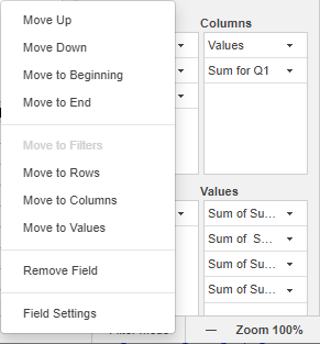
Once the fields are added to the necessary sections, you can manage them to change the layout and format of the pivot table. Click the black arrow to the right of a field within the Filters, Columns, Rows, or Values sections to access the field context menu.
-
Move the selected field Up, Down, to the Beginning, or to the End of the current section if you have added more than one field to the current section.
-
Move the selected field to a different section - to Filters, Columns, Rows, or Values. The option that corresponds to the current section will be disabled.
-
Remove the selected field from the current section.
-
Adjust the selected field settings.
The Filters, Columns, and Rows field settings look similarly:

The Layout tab contains the following options:
-
The Source name option allows you to view the field name corresponding to the column header from the source data set.
-
The Custom name option allows you to change the name of the selected field displayed in the pivot table.
-
The Report Form section allows you to change the way the selected field is displayed in the pivot table:
-
Choose the necessary layout for the selected field in the pivot table:
-
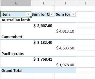
The Tabular form displays one column for each field and provides space for field headers.
-
The Outline form displays one column for each field and provides space for field headers. It also allows you to display subtotals at the top of groups.
-
The Compact form displays items from different row section fields in a single column.
-
-
The Repeat items labels at each row option allows you to visually group rows or columns together if you have multiple fields in the tabular form.
-
The Insert blank rows after each item option allows you to add blank lines after items of the selected field.
-
The Show subtotals option allows you to choose if you want to display subtotals for the selected field. You can select one of the options: Show at top of groupor Show at bottom of group.
-
The Show items with no data option allows you to show or hide blank items in the selected field.
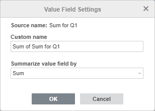
Value field settings
-
The Source name option allows you to view the field name corresponding to the column header from the source data set.
-
The Custom name option allows you to change the name of the selected field displayed in the pivot table.
-
The Summarize value field by list allows you to choose the function used to calculate the summation value for all values from this field. By default, Sumis used for numeric values, Countis used for text values. The available functions are Sum, Count, Average, Max, Min, Product, Count Numbers, StdDev, StdDevp, Var, Varp.
Change the appearance of pivot tables
-
The Report Layoutdrop-down list allows you to choose the necessary layout for your pivot table:
-
Show in Compact Form: allows you to display items from different row section fields in a single column.
-
Show in Outline Form: allows you to display the pivot table in the classic pivot table style. It displays one column for each field and provides space for field headers. It also allows you to display subtotals at the top of groups.
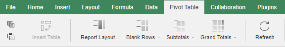
Change the appearance of pivot tables
You can use options available on the top toolbar to adjust the way your pivot table is displayed. These options are applied to the entire pivot table.
Select at least one cell within the pivot table with the mouse to activate the editing tools on the top toolbar.
-
The Report Layout drop-down list allows you to choose the necessary layout for your pivot table:
-
Show in Compact Form: allows you to display items from different row section fields in a single column.
-
Show in Outline Form: allows you to display the pivot table in the classic pivot table style. It displays one column for each field and provides space for field headers. It also allows you to display subtotals at the top of groups.
-
Show in Tabular Form: allows you to display the pivot table in a traditional table format. It displays one column for each field and provides space for field headers.
-
Repeat All Item Labels: allows you to visually group rows or columns together if you have multiple fields in the tabular form.
-
Don't Repeat All Item Labels: allows you to hide item labels if you have multiple fields in the tabular form.
-
-
The Blank Rowsdrop-down list allows you to choose if you want to display blank lines after items:
-
Insert Blank Line after Each Item: allows you to add blank lines after items.
-
Remove Blank Line after Each Item: allows you to remove the added blank lines.
-
-
The Subtotalsdrop-down list allows you to choose if you want to display subtotals in the pivot table:
-
Don't Show Subtotals: allows you to hide subtotals for all items.
-
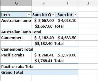
Show all Subtotals at Bottom of Group: allows you to display subtotals below the subtotaled rows.
-
Show all Subtotals at Top of Group: allows you to display subtotals above the subtotaled rows.
-
-
The Grand Totals drop-down list allows you to choose if you want to display grand totals in the pivot table:
-
Off for Rows and Columns: allows you to hide grand totals for both rows and columns.
-
On for Rows and Columns: allows you to display grand totals for both rows and columns.
-
On for Rows Only: allows you to display grand totals for rows only.
-
On for Columns Only: allows you to display grand totals for columns only.
-
Note: The similar settings are also available in the pivot table advanced settings window in the Grand Totals section of the Name and Layout tab.
The  Select button allows you to select the entire pivot table.
If you change the data in your source data set, select the pivot table and click the  Refresh button to update the pivot table.
Change the style of pivot tables
You can change the appearance of pivot tables in a spreadsheet using the style editing tools available on the top toolbar.
Select at least one cell within the pivot table with the mouse to activate the editing tools on the top toolbar.
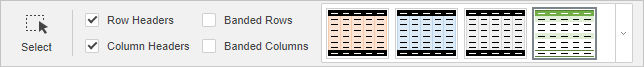
-
Row Headers: allows you to highlight the row headers with special formatting.
-
Column Headers: allows you to highlight the column headers with special formatting.
-
Banded Rows: enables the background color alternation for odd and even rows.
-
Banded Columns: enables the background color alternation for odd and even columns.
The template list allows you to choose one of the predefined pivot table styles. Each template combines certain formatting parameters, such as a background color, border style, row/column banding, etc. Depending on the options checked for rows and columns, the templates set will be displayed differently. For example, if you've checked the Row Headers and Banded Columns options, the displayed templates list will include only templates with the row headers highlighted and banded columns enabled.
Filter, sort and add slicers in pivot tables
You can filter pivot tables by labels or values and use the additional sort parameters.
Filtering
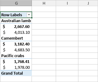
Click the dropdown arrow  in the Row Labels or Column Labels of the pivot table. The Filter option list will open:
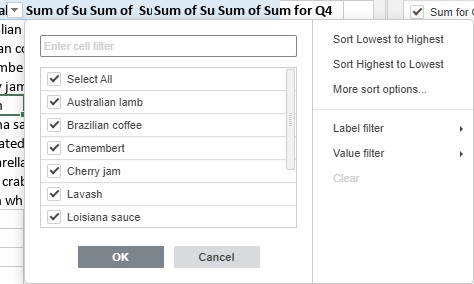
Adjust the filter parameters. You can proceed in one of the following ways: select the data to display or filter the data by certain criteria.
-
Select the data to display
Uncheck the boxes near the data you need to hide. For your convenience, all the data within the Filter option list are sorted in ascending order.
Note: The (blank) checkbox corresponds to the empty cells. It is available if the selected cell range contains at least one empty cell.
To facilitate the process, make use of the search field on the top. Enter your query, entirely or partially, in the field - the values that include these characters will be displayed in the list below. The following two options will be also available:
-
Select All Search Results: is checked by default. It allows selecting all the values that correspond to your query in the list.
-
Add current selection to filter: if you check this box, the selected values will not be hidden when you apply the filter.
After you select all the necessary data, click the OK button in the Filteroption list to apply the filter.
-
Filter data by certain criteria
You can choose either the Label filter or the Value filter option on the right side of the Filteroptions list, and then select one of the options from the submenu:
-
For the Label filterthe following options are available:
-
For texts: Equals...,Does not equal..., Begins with...,Does not begin with..., Ends with...,Does not end with..., Contains...,Does not contain...
-
For numbers: Greater than...,Greater than or equal to..., Less than...,Less than or equal to..., Between,Not between.
-
-
For the Value filter the following options are available: Equals...,Does not equal..., Greater than...,Greater than or equal to..., Less than...,Less than or equal to..., Between,Not between, Top 10.
-
The Filter  button will appear in the Row Labels or Column Labels of the pivot table. It means that the filter is applied.
Sorting
You can sort your pivot table data using the sort options. Click the dropdown arrow in the Row Labels or Column Labels of the pivot table and then select Sort Lowest to Highest or Sort Highest to Lowest option from the submenu.
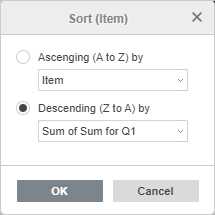
The More Sort Options option allows you to open the Sort window where you can select the necessary sorting order - Ascending or Descending: and then select a certain field you want to sort.
Adding slicers
You can add slicers to filter data easier by displaying only what is needed.
Adjust pivot table advanced settings
To change the advanced settings of the pivot table, use the Show advanced settings link on the right sidebar. The 'Pivot Table - Advanced Settings' window will open:
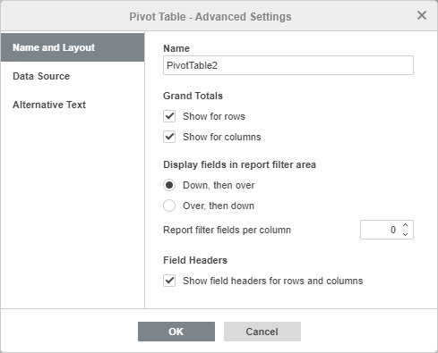
The Name and Layout tab allows you to change the pivot table common properties.
-
The Name option allows you to change the pivot table name.
-
The Grand Totals section allows you to choose if you want to display grand totals in the pivot table. The Show for rowsand Show for columnsoptions are checked by default. You can uncheck either one of them or both these options to hide the corresponding grand totals from your pivot table.
Note: The similar settings are available on the top toolbar in the Grand Totalsmenu.
-
The Display fields in report filter area section allows you to adjust the report filters which appear when you add fields to the Filters section:
-
The Down, then over ;option is used for column arrangement. It allows you to show the report filters across the column.
-
The Over, then down option is used for row arrangement. It allows you to show the report filters across the row.
-
The Report filter fields per column option allows you to select the number of filters to go in each column. The default value is set to0. You can set the necessary numeric value.
-
-
The Field Headers section allows you to choose if you want to display field headers in your pivot table. The Show field headers for rows and columnsoption is selected by default. Uncheck it to hide field headers from your pivot table.
-
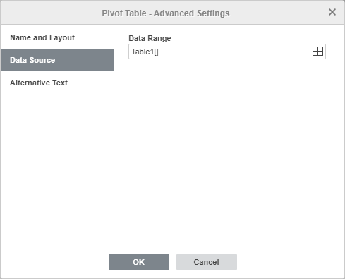
The Data Source tab allows you to change the data you wish to use to create the pivot table.
Check the selected Data Range and modify it, if necessary. To do that, click the icon .
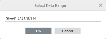
In the Select Data Range window, enter the necessary data range in the following format: Sheet1!$A$1:$E$10. You can also select the necessary cell range in the sheet using the mouse. When ready, click OK.
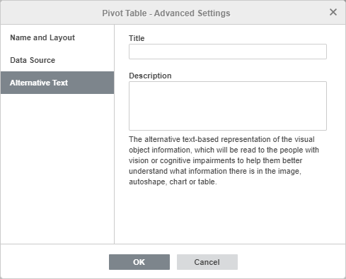
The Alternative Text tab allows specifying the Title and the Description which will be read to people with vision or cognitive impairments to help them better understand what information the pivot table contains.
Delete a pivot table
To delete a pivot table,
-
Select the entire pivot table using the
Selectbutton on the top toolbar. -
Press the Delete key.

